Overfitting in Deep Learning and Ways to Reduce It

Assume that in a particular class the teacher gave a set of sample questions and answers on the materials he/she covered during the course. There are three students in the class, A, B, and C. A is not much interested in learning. B memorized all the questions and answers than trying to understand them. Even if the teacher mistakenly gave a wrong sample answer to a particular question, B memorized that too without having a proper understanding. But, C tried to understand each and every question and the answers than just memorizing them. When the teacher conducted an exam by repeatedly giving the same questions he/she gave during the course, B gets the highest marks as he memorized the answers for those questions. A gets the lowest marks as he didn’t study. On the other hand, C gets reasonably good marks, but may not be the highest one. However, when the teacher gave a new set of questions, A will definitely get the lowest marks, and B also will receive a very low marks as he only memorized the previous set of questions and answers and not prepared for the new sets of questions. But C will get good marks even for this new set of questions as he “generalized” well. This scenario explains the three terms: “underfitting”, “overfitting”, and a “good-fit” in machine learning. Here, A is a good example for “underfitting” – a problem in machine learning where the machine learning model can neither learn from the training data nor generalize to new data. Underfitting can be solved by increasing the complexity of the machine learning model. B is a good example for “overfitting” – another problem in machine learning, where the machine learning model tries to remember the training data than trying to learn from it. On the other hand, C is the good example for a “good fit” – a preferred machine learning solution.

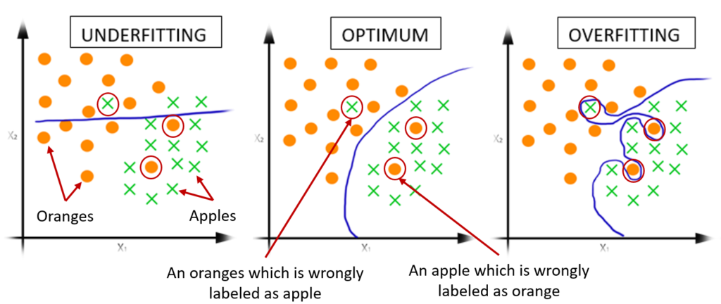
Figure 1: Illustration of underfitting, optimum-fit, and overfitting for the classification of apples vs oranges. A machine learning model is learned to separate these two classes. The separation boundary is shown in blue. In underfitting the model does not find a good separation. In the optimum case (good-fit) a preferred solution is found, which is even robust to some degree of noisy labels. In overfitting, the model fits to all the data points including the noisy data points.

Similarly, assume that you are training a deep learning model, and the model perfectly fits your training data and gives you a high prediction score on it. But when you apply that trained model to unseen test data you get worse predictions (similar to the student B). This explains the problem of overfitting in Machine/Deep Learning. When a model overfits the training data, it tries to memorize the patterns of the training data than generalize to unseen test data which is drawn from the same distribution as the one used to generate the model. Figure 1 illustrates this scenario using a toy example.

As overfitting is one of the major problems in deep learning, there are various approaches explored to reduce it. These approaches range from increasing the amount of training data to improving the way deep learning models are trained. The following sections summarize these methods.

1. Increase the amount of training data by Data Augmentation: Deep learning models are usually data-hungry, meaning that they require a large amount of data for training as they contain millions of parameters to tune. If the model is trained using a small amount of data, it can severely overfit by just remembering each of the training samples than learning from it. Collecting a large amount of labeled data for training is often a tedious, time-consuming task, and requires expert knowledge. To overcome this, data augmentation techniques are widely used as a way to increase the amount of training data, where, the original data is somehow transformed into new additional data, and the deep learning model is then trained on this augmented (original and the newly created) data. Various such transformations could be used, for example, in the case of images, rotations, scaling, cropping, flipping, are named a few. Generative models, such as Generative Adversarial Networks (GANs) and Auto-encoders were also explored as an alternate for data augmentation as they can generate new data (Sandfort et. al., 2019). Adding random noise to the input data, every time the data is loaded for training also can be considered as a way of data augmentation.

In most cases, data augmentation alone is not enough to reduce overfitting. The network should be carefully trained, particularly when we have a lack of training data.

2. Transfer learning: Deep learning models usually contain millions of parameters and require a large amount of data to learn them, and if it is unavailable the trained model will lead to overfitting. A good initialization of these parameters often leads to better convergence in training the deep models and can reduce overfitting. Transfer learning is a widely used technique to transfer the knowledge learned on a particular task to improve the performance on a different, but a relative task. In transfer learning, the weights of the learned network on a particular task are used to initialize the weights of the current network for the task under consideration.

3. Simplify the Network: Usually larger networks give better performance than the smaller ones, particularly when you train them with enough data. However, when you train a large network on a small amount of data, the network will try to remember each instance of the training data than ‘learning’ from data. Therefore, by reducing the complexity of the network overfitting can be reduced. The easiest way to reduce the network complexity is to reduce the number of parameters it contains by reducing the number of layers and/or the number of neurons at each layer.

4. Early stopping: In deep learning, the deep neural network is trained iteratively to update the network parameters such that the error on the training data is reduced. Over the iterations, the error is reduced and the network’s prediction performance increases. However, overtraining is often leads to overfitting. Therefore, to avoid the network from overtraining early stopping is necessary. One way to decide when to stop training is the use of a validation set; The training could be stopped when the performance on the validation set no longer increases or tends to decrease.

5. Weight regularization: Without weight regularization, the weights of the network may become arbitrarily large. Regularization (also called weight decay) penalizes large weights by adding a constraint on the loss function which is used to train the network. The loss function now contains two terms, the first one tries to minimize the training error on the training data and the second one is the regularization term for penalizing larger weights.

6. Introduce randomness and/or noise in training: Randomness can be incorporated or noise could be added at the training stage of the network to avoid the network from memorizing the training data. Various such techniques exist, including Noise injection, Stochastic Pooling (Zeiler et. al., 2013), Drop-out (Srivastava et. al., 2014), Drop-Connect (Wan et. al., 2013).

In the case of noise injection, random noise is added to the network nodes and/or to the input data at each iteration of training. This enables the network robust against noise and small variations in the input data.

Stochastic pooling is a pooling technique that applies randomness at the training stage of the network. Unlike other deterministic pooling approaches (e.g., max or average pooling) where all the activations inside each pooling region are considered when pooling, in Stochastic pooling the activations within each pooling region are randomly picked based on a multinomial distribution given by the values within that pooling region. In testing, no randomness is included, and all the activations are considered with a weighting scheme. Some other pooling approaches for this purpose include S3 pooling (Zhai et. al., 2017), mixed max-average pooling.

Drop-out is a widely used technique to reduce overfitting, where hidden nodes of the network are randomly dropped at each iteration of training. As different sets of nodes are dropped at different iterations, training at a particular iteration is more like training a thinned version of the original network. Therefore, training a network using Drop-out can be viewed as training a network ensemble. Although Drop-out is a simple and widely used approach it introduces an additional parameter (the percentage of the nodes that should be dropped) and it may take longer to train compared to a network without dropout (Srivastava et. al., 2014). At the prediction time, no dropout is used. Drop-connect is similar to Drop-out. But in Drop-connect instead of dropping hidden nodes, some connections (weights) are randomly set to zero.

7. Use validation data: The main question about overfitting is how do we know when the model starts to overfit? A validation dataset could be used for this purpose. Over the training iterations, the model could be periodically tested on this validation dataset. When there is no improvement in the performance score on the validation dataset, or when the validation score starts to decrease the training could be stopped or any other appropriate action could be taken, e.g., reduce the learning rate. The validation dataset also can be used to identify the appropriate value(s) of the free parameter(s) of the model. For example, if the loss function contains two or more terms, the trade-off parameter(s) of different terms of the loss could be selected in a way that the selected parameter(s) leads/lead to the best validation score.

8. Ensembling: Ensembling is an approach where a set of deep learning models are trained and their outputs for a given sample are combined (e.g., by averaging, majority voting) as the final prediction for that sample. Ensembling not only reduces overfitting but also reportedly produces improved performance than a single model (Garbin et. al., 2020). However, training an ensemble takes much more time than training a single model.

9. Penalize over-confident predictions: These methods focus on regularizing the output distributions of the network so that the network can generalize well. Label-Smoothing (Pereyra et. al., 2017) is a well-known approach for this purpose, although it can be done using different other approaches. In classification problems, we generally use ‘hard labels’. The loss based on these hard labels encourages the network to provide a high-confident prediction for each sample, and this can lead to overfitting. Label-smoothing is a simple technique that reduces the problems of both overfitting and over-confident predictions by the use of soft labels than the hard-ones.

10. Batch normalization: Batch normalization (Loffe et. al., 2015) improves the speed, performance, stability, and generalization ability of the network by normalizing the input of each layer to have zero mean and a unit standard deviation. Overfitting is reduced as batch normalization acts as a regularizer and improves the generalization ability of the network.

References

Garbin, C., Zhu, X. & Marques, O., 2020 Dropout vs. batch normalization: an empirical study of their impact to deep learning. Multimedia Tools Applications, 79, 12777–12815.

Loffe S., & Szegedy C., 2015 Batch normalization: accelerating deep network training by reducing internal covariate shift. International Conference on Machine Learning, 37, 448–456.

Pereyra G., Tucker G., Chorowski J., Kaiser L., & Hinton G. E., 2017 Regularizing Neural Networks by Penalizing Confident Output Distributions, International Conference on Learning Representations (workshop).

Sandfort, V., Yan, K., Pickhardt, P.J. et al. (2019) Data augmentation using generative adversarial networks (CycleGAN) to improve generalizability in CT segmentation tasks. Nature Scientific Reports 9, 16884

Srivastava N., Hinton G., Krizhevsky A., Sutskever I., Salakhutdinov R., 2014 Dropout: A Simple Way to Prevent Neural Networks from Overfitting, Journal of Machine Learning Research 15,1929-1958

Wan L., Zeiler M., Zhang S., Cun Y.L., Fergus R; 2013 Regularization of Neural Networks using DropConnect, International Conference on Machine Learning, 28(3):1058-1066

Zhai, S., Wu, H., Kumar, A., Cheng, Y., Lu, Y., Zhang, Z., & Feris, R. (2017). S3Pool: Pooling with Stochastic Spatial Sampling. IEEE Conference on Computer Vision and Pattern Recognition, 4003-4011.

Zeiler M., & Rob F., (2013). Stochastic Pooling for Regularization of Deep Convolutional Neural Networks, International Conference on Learning Representations.